Loading and Viewing Raw Data
Loading Raw Data
Data sets stored in the application’s native format can be opened using the Dataset→Open... menu
item. Note that the native format is actually a zarr directory
tree, and not an individual file. These data directories can be identified by the .tr.zarr
suffix to their names.
Data stored in other formats can be imported using the Dataset→Import→Raw Data... menu item.
Currently, comma-separated values (.csv) files and the proprietary .ufs format from
Ultrafast Systems are supported. Multiple files may be loaded at once which represent multiple scans
of the same sample for averaging.
For .csv formatted files, the first row should contain the time axis labels, and the first column
should contain the wavelength axis labels.
Example .ufs files are available on the web here.
Navigation
Typical time-resolved dataset contains multidimensional data, for example, intensity as a function of wavelength, time, and scan number. The raw data is plotted in several panels to help view this through “slices” through the different dimensions.
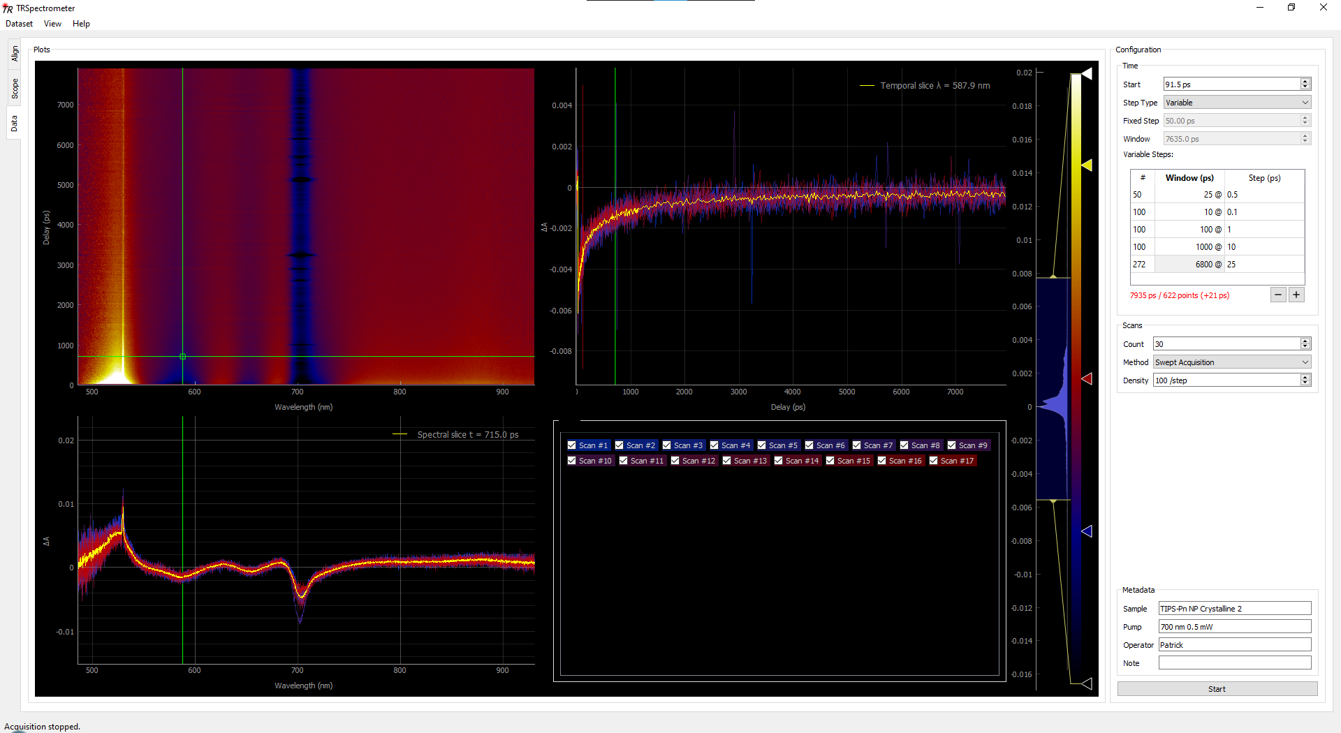
Data panel of the software showing some raw data.
In the example image above, the plot panels are:
Upper-left: the complete data set as a “heatmap” image, built using the average of all the selected scans. This shows the change-in-absorbance (ΔA) signal as a function of wavelength and pump–probe delay time.
Upper-right: the “temporal slice”, which plots slices through the data set at one selected wavelength. The wavelength selection is performed using the green crosshairs in either the upper-left or lower-left panels. Each scan is plotted in a different colour, and the average of the selected scans in plotted in yellow.
Lower-left: the “spectral slice”, which plots slices through the data set at one selected time. The time selection is performed using the green crosshairs in either the upper-left or upper-right panels. Each scan is plotted in a different colour, and the average of the selected scans in plotted in yellow.
Colour bar: a vertical histogram shows the distribution of the intensity values. The dark blue selection region chooses the intensity range to use for the colour map. The colour map can be modified using the arrows to the right of the colour bar, or by right-clicking the colour bar itself.
Lower-right: A series of check boxes can be used to select which scans are displayed and used in the averaging of the data set. The background colour of the check box is the same as its respective trace in the plot panels. Hovering the mouse over a check box will highlight the corresponding traces in white. Conversely, clicking on a trace in the temporal or spectral slice plots will highlight the corresponding check box.

Selecting scans to be used in averaging of the data set. Note the white highlighting of the traces which correspond to the check box currently being pointed at with the mouse.
Use the mouse to interact with the plot areas:
Left mouse button:
Drag elements such as the crosshairs (green lines).
Select traces in the temporal or spectral slice panels.
Drag the plot area to pan along both axes.
Drag axis labels to pan along only that single axis.
Right mouse button:
Drag the plot areas to zoom in both axes.
Drag axis labels to zoom in only that single axis.
Middle mouse button (wheel click):
Drag the plot area to pan. As the left button, but ignores elements like the crosshairs.
Mouse wheel:
Scroll on plot areas to zoom in both axes.
Scroll on axis labels to zoom in only that single axis.
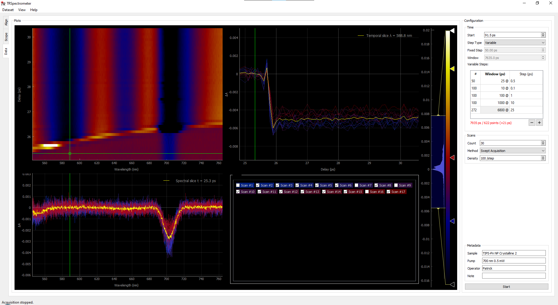
View of the raw data when zoomed in to a small section of the data set. This section is around the time zero.
The plot areas are linked, in that a change in the zoom or pan of one plot will be mirrored in the other panels.
Note that zooming occurs around the location of the mouse pointer. That is, the plot will zoom in to where the pointer is.
Small 🄰 buttons appear at the lower-left corner of each plot panel. Clicking them will return to an “auto” zoom mode which will attempt to display the entire data set.
Saving Raw Data
Data can be saved in the application’s native format using the Dataset→Save As... menu item.
Note that the native format is actually a zarr directory tree, and
not an individual file. These data directories will have the .tr.zarr suffix appended to their
names.
An average of the selected scans can be saved using the Dataset→Export→Raw Data Average... menu
item. Both comma-separated values (.csv) and the proprietary .ufs format from Ultrafast
Systems are supported. These exported data formats are useful for analysis in other software
packages such as Glotaran or Surface Xplorer.