Configuring Acquisition Parameters

There are no hard rules about what the “correct” acquisition parameters are. The selection is usually a balance between signal-to-noise versus acquisition time, data resolution versus disk and memory space (and acquisition time) etc. The general goal is to capture any rapidly changing dynamics of the sample with sufficient time resolution (such as around time zero), but use reduced sampling at later times when the sample dynamics evolve more slowly. Some sampling before time zero is also desirable to evaluate the level of background signal from pump scattering or spontaneous emission etc.

Here, we will show an example of how some acquisition parameters might be chosen. Remember however, this is just an example and you should use your own judgement about what parameters will meet your needs and are physically possible on the equipment.

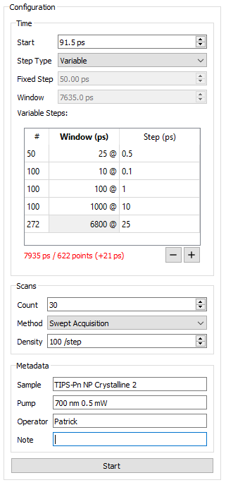
Configuration section of the Data panel with example parameters entered.

Time Section

After completing the Alignment process, the “time zero” should be known. This is the absolute delay time when the pump and probe beams arrive on the sample simultaneously and the signal is just beginning to appear. For this example, the time zero was found to be at 117.5 ps. We decide to sample 25 ps of background. We also want a little bit of leeway before the signal begins to appear, so we set the Start parameter to 26 ps before time zero, or 91.5 ps.

We choose a Step Type of Variable, since we want to be able to have better time resolution around time zero than the bulk of the data set. Choosing the alternative Fixed step mode with a large step size may be appropriate for initial scans to quickly get an idea of the sample behaviour.

For a variable step type, the Variable Steps table needs to be filled in. Each row in the table represents a time step range. The columns are the number of steps (or data points) for the range, the time window of the range, and the step size (resolution) of the range. Only the second and third columns are editable, while the number of steps will be computed from the window size and resolution. Use the + and - buttons below the table to add rows to the table, or remove the currently selected row.

We already decided we wanted 25 ps of background data before time zero, so the first row in the table has a window of 25 ps. A resolution of 0.5 ps is selected to give 50 time points in this region. This is quite generous, but a good rule is to collect at least 10 data points here.

The second step range should capture the rapid dynamics of the system around time zero. The window needs to be wide enough to see the signal rise across the full spectral window, taking into consideration the instrument response time and chirp (temporal dispersion) in the probe light, as well as any rapid changes in the sample directly after excitation. As the resolution needs to be quite high over this region, it’s also desirable to have this window be the smallest possible to avoid collecting an excessive amount of data in this region. We choose a 10 ps window with a resolution of 100 fs to give 100 data points in this region.

The subsequent step ranges are somewhat arbitrarily chosen so that the next 100 ps of data are collected with 1 ps resolution followed by 1 ns at 10 ps resolution, giving 100 data points in each of those ranges. Finally, we know this particular sample has a long-lived species present, so we run the final step range out to the limits of what is possible with the installed delay hardware with a resolution of 25 ps. The selected window of 6.8 ns is enough to exceed the limits of the delay by 21 ps, indicated by the red highlight and (+21 ps) in the totals displayed below the table.

The numbers directly below the table provide the sum total of the sampling window, as well as the total number of time points. The number of points will have a direct impact on both the data acquisition time, and storage space required. If the sampling window will exceed the capabilities of the delay hardware (also taking into consideration the start time), this display will be highlighted in red. The window will be truncated automatically during the acquisition process. The excess time window is given in parenthesis. In this example, the +21 ps excess will cause the final delay range to actually be 6779 ps instead of the requested 6800 ps.

Scans Section

The Count value determines how many repeats of the acquisition process should be performed. The individual scans will be averaged which helps improve signal-to-noise, particularly compensating for longer-term fluctuations such as pump laser power drift, slight alignment changes due to air conditioning cycles or similar. It will also help smooth over “blips” which may be caused by momentary scattering from particles in a solution sample, or accidental bumps on the equipment. The number of scans can be adjusted during the acquisition process, so it can be good to initially set this value much higher than expected, then dial it down to stop the acquisition process when the quality of data begins looking good enough.

The Method selects the strategy used to acquire the data. The available choices will depend on the acquisition Plugins which are loaded and their particular Configuration. We have selected Swept Acquisition here. The swept acquisition is highly recommended if the hardware is capable of this mode. The more traditional stepped acquisition should be available to all hardware types but will be much slower for the same data quality.

The Density parameter selects the desired number of samples performed at each time step of each scan. In this example, a value of 100 means to take 100 ΔA measurements (200 laser shots) and average them for each time point. For a swept acquisition method, this determines how fast the delay is swept and has an approximately linear proportionality to the acquisition time. In this case it is suggested to use a relatively low density (50 to 200 per step) but a large (10 to 50) number of scans. For a stepped acquisition method, significant amounts of time are spent moving the delay into position (and not actually sampling data), therefore it is optimal to do more sampling at each step (200 to 500 per step), but a smaller number of scans will be possible (3 to 10) within a reasonable time frame.

Metadata Section

Metadata is “data about the data”. These fields are completely optional, but worth filling out for the benefit of any future users of the data, which are likely to be you!

The Sample field can be used for the name of the sample. It will be used as part of the suggested file name when the data is saved.

The Pump field should be used to describe the nature of the pump laser, such as its wavelength, pulse energy, and polarisation. It will also be used as part of the suggested file name when the data is saved.

Operator should be the name(s) of the people collecting the data.

Note can be any additional information about the sample, equipment, conditions etc which might be relevant.